Differential Pressure Flow Meters: Principles, Installation, and Applications - Just Measure it

Differential Pressure Flow Meters: Principles, Installation, and Applications

1. Principle of Differential Pressure Flow Measurement

When a fluid completely fills a pipeline and flows through a primary element (such as an orifice plate or nozzle), a local constriction is created. This results in an increase in velocity and a decrease in static pressure. Consequently, a differential pressure (DP) forms before and after the constriction. The larger the flow rate, the greater the DP generated. By measuring this pressure difference, the flow rate can be accurately determined.

Pressure Transmitter

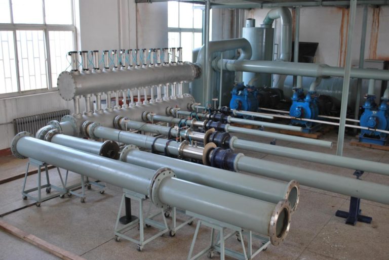
2. Basic Installation Requirements for Throttling Devices

  1. Verify the model and dimensions of the throttling device before installation to ensure compatibility with the pipeline location.

  2. For new piping systems, install the device only after flushing the pipeline.

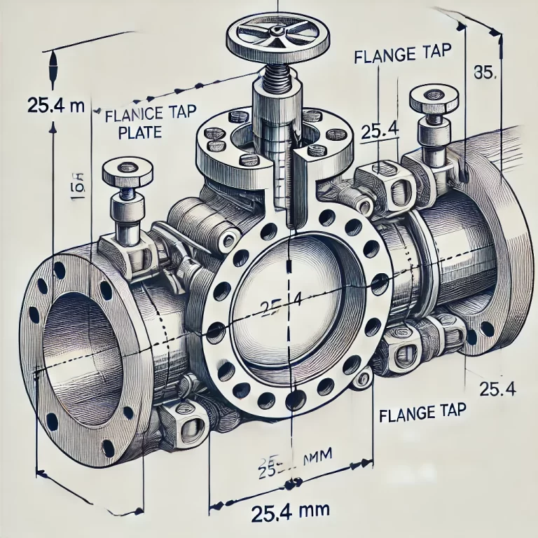
  3. Observe the correct installation direction—marked with a “+” symbol on the upstream side.

  4. Ensure perpendicularity and concentricity with the pipeline. Perpendicularity error should not exceed ±1°, and concentricity deviation should be within 0.0025D or 0.1 + 2.3B4.

  5. Gaskets must not protrude into the pipe interior.

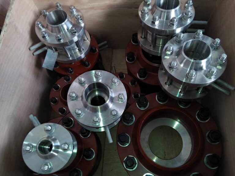
  6. The orifice assembly must be leak-proof; pressure testing is required after installation.

  7. Impulse lines should be installed vertically or at an incline (minimum 1:12 gradient). For viscous fluids or long distances (>3m), install gas traps or sediment pots at the highest and lowest points.

  8. Keep high and low pressure impulse lines close together to reduce signal distortion. In cold regions, use insulation or heat tracing.

  9. Proper tap location is essential. For vertical pipes, tapping can be on any side; for horizontal pipes, specific positioning is recommended.

  10. Observe required straight pipe lengths upstream (L1) and downstream (L2), based on multiples of pipe diameter (D).

3. Impulse Line Layouts

Provide proper impulse line arrangements for different media:

  • Clean Liquids

  • Corrosive Liquids

  • Clean Gases

  • Corrosive Dry Gases

  • Steam

Each configuration has unique layout requirements to ensure accurate pressure transmission.

4. Flow Calculation Formulas

Mass Flow (M):

M = C × A × √(ΔP / ρ)

Volumetric Flow (V):

V = C × A × √(ΔP / ρ)

Where:

  • C: Flow coefficient

  • A: Area of orifice opening (πd²/4)

  • ΔP: Differential pressure (Pa)

  • ρ: Fluid density (kg/m³)

  • d: Orifice diameter (m)

  • D: Pipe inner diameter (m)

  • β: Diameter ratio (d/D)

Temperature and Pressure Compensation:

  • Gas Compensation:

    Q_comp = Q_meas × (P_meas / P_design) × (T_design / T_meas)

  • Steam Compensation:

    • For saturated steam: pressure-based compensation is typically used.

    • For superheated steam:

      M_comp = M_meas × (ρ_design / ρ_actual)

5. Balanced Flow Meter (Multi-Hole Design)

  • Structure: Symmetrical multi-hole layout balances the flow field, reduces turbulence, vibration, and signal noise.

  • Advantages:

    • Low straight pipe requirements (e.g., 3D upstream, 2D downstream).

    • Low permanent pressure loss.

    • Anti-clogging design reduces stagnant zones.

    • Applicable to gas, liquid, steam, and high-temp/high-pressure conditions.

  • Specifications:

    • Pipe size: DN15–DN3000

    • Pressure: 0.25–42 MPa

    • Temp: -200 to 600°C

    • Accuracy: 0.5–2%

6. V-Cone Flow Meter

  • Principle: Based on Bernoulli’s theorem. The V-cone constricts the flow at the center, creating a DP between upstream and downstream tap points.

  • Specs:

    • DN25–DN2000

    • Pressure up to 10 MPa

    • Temp: -200 to 500°C

    • Accuracy: ±1%

  • Straight Pipe Requirements:

    • 5–10D upstream, 2–3D downstream

  • DP Transmitter Positioning:

    • Below the V-cone for liquids and steam

    • Above the V-cone for gases


7. Nozzles (ISA1932 and Long Radius)

  • Principle: Like orifice plates, nozzles create DP by accelerating flow.

  • Features:

    • Less pressure loss than orifice plates

    • Suitable for high-temp, high-pressure applications

    • High accuracy and repeatability

  • Types:

    • ISA1932: Arc-shaped converging section

    • Long Radius: For β = 0.25–0.80; uses radial tapping

Flow Formula Example:

M = K × d² × ε × α × √(ΔP / ρ)
  • K: Constant based on unit system

  • ε: Expansion coefficient

  • α: Discharge coefficient

8. Anti-Clog Array Airflow Measurement System

  • Install at: 20D upstream, 5D downstream straight pipe preferred

  • Connection: All sensor probes’ positive/negative sides should be connected before linking to the DP transmitter

  • Calibration Port: ≥200 mm upstream or ≥500 mm downstream, diameter ≥50 mm

Compensation Formula:

Qv = k × A × √(Pd / (ρ × (1 + t / 273.15)))


9. Primary Airflow Measurement with Pitot Tubes

  • Principle: Measures total vs static pressure to determine velocity

  • Installation:

    • Vertical mounting on horizontal pipes

    • Facing into airflow direction

    • Straight pipe: 20D upstream, 5D downstream

Velocity Calculation:

V = k × √(2 × Pd / ρ)
  • k: Coefficient (initial 0.83)

  • Pd: Differential pressure

  • ρ: Fluid density (based on temp and pressure)

Share This Story, Choose Your Platform!

Contact Us

    Please prove you are human by selecting the heart.
    Translate »