In engineering and scientific fields, “signals” typically refer to a function that conveys information through variation with respect to some independent variable, most commonly time. The function’s values can represent physical quantities such as voltage, current, light intensity, sound pressure, or electromagnetic field strength.
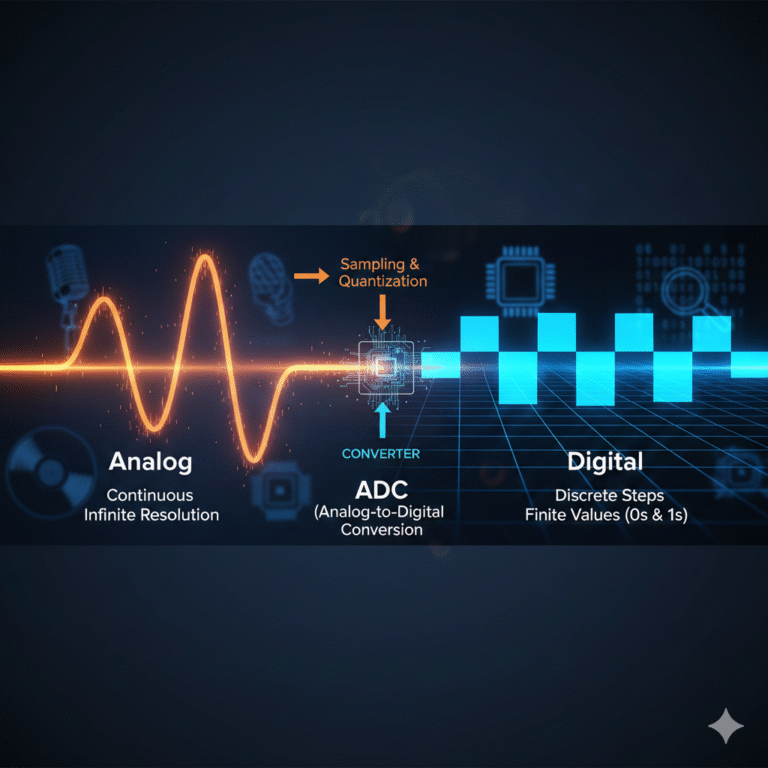
Analog Signals
An analog signal is one that varies continuously in both time and amplitude. The core feature of analog signals is their continuity in two aspects:
Time Continuity: Between any two time points, theoretically, an infinite number of moments can be inserted.
Amplitude Continuity: The values of the signal can be infinitely subdivided within a range, with no minimum unit.
Most signals directly generated by the real world (such as the sound pressure voltage output from microphones, raw outputs from sensors like temperature, pressure, and displacement, or electromagnetic wave signals received by antennas) are analog. In mathematical terms, these signals can be perfectly modeled by continuous functions.
Analog signals are highly susceptible to noise interference. Since their values are infinitely divisible, even the slightest noise can alter the original value, and such changes are often irreversible and cumulative during transmission.
Digital Signals
A digital signal is not naturally occurring; rather, it is a symbolic representation designed by humans to simplify storage, computation, and transmission. A digital signal’s values come from a finite set. Inside computers, it is represented as a binary sequence (0s and 1s), and in communication links, it may appear as a limited number of discrete voltage levels or phase states.
For example, the sample data in audio files, pixel values from image sensors, internal logic signals in processors and FPGAs, and bitstreams in network communication are all digital signals.
The shift to digital signals isn’t because they are “more real” than analog signals, but because they offer determinism. Digital signals use threshold-based decision-making to combat noise— as long as the noise is not strong enough to misinterpret a 0 as 1, the information can be restored 100%.
Understanding this distinction helps in appreciating the relationship between analog and digital signals.
Differences Between Analog and Digital Signals
There’s no simple “better or worse” comparison between analog and digital signals. Rather, their characteristics differ in the following ways:
Continuity vs. Discreteness
Analog signals are continuous in both time and amplitude, capable of describing minute changes.
Digital signals are discrete in either time or amplitude, with precision determined by the sampling rate and quantization.
Noise Behavior
In analog systems, noise directly adds to the signal’s amplitude. As such, the quality of analog signals tends to degrade gradually.
In digital systems, noise primarily affects decision results, manifesting as bit or symbol errors. The quality of digital signals is measured by the likelihood of errors.
Transmission and Replication
Analog signals tend to accumulate errors when amplified, transmitted, or replicated.
Digital signals can be restored to their standard form through decision-making and reconstruction, making them more reliable over long distances and in large-scale systems.
Processing Differences
Analog signal processing relies on continuous circuits like amplifiers, filters, and mixers, which are influenced by the physical characteristics of the devices.
Digital signal processing depends on clocks, logic circuits, and algorithms, which are shaped by system structure and algorithm design.
From Analog to Digital: What Changes?
Since most real-world signals are analog, but subsequent processing is often done digitally (such as by processors or FPGAs), a “conversion process” is required. Analog-to-digital conversion (ADC) becomes a crucial step.
Basic Steps of ADC
Sampling
Sampling is the process of taking an instantaneous value at regular intervals on a continuous timeline.Sampling Rate: The number of samples taken per second.
Sampling Theorem: A signal must be sampled at least twice the highest frequency to be theoretically reconstructed without distortion.
Quantization
After sampling, the values are still continuous in amplitude. Quantization maps them into a finite set of levels.Quantization Noise: The rounding or “rounding off” during quantization introduces a small error between the quantized value and the original value, known as quantization noise.
Encoding
The quantized results are then converted into binary or another digital format for processing by digital systems.
These three steps together determine how well the digital signal can represent the original analog signal. The ability to describe the signal well depends on the application’s needs and system goals.

Sampling Rate Significance
In practical systems, the choice of sampling rate is more critical than it may seem. This relates to how the signal behaves in the frequency domain.
Sampling Theorem
According to the Nyquist-Shannon Sampling Theorem, if a signal’s sampling frequency is at least twice its maximum frequency, the signal can be ideally reconstructed with proper processing.Aliasing Phenomenon
When the sampling frequency is insufficient, high-frequency components “fold” into the lower-frequency region, causing different frequencies to become indistinguishable and resulting in aliasing. Once aliasing occurs, original frequency spectrum information is lost, and further processing can only work with the incorrect representation.
To prevent aliasing, engineers typically add an analog anti-aliasing filter (AAF) before the ADC to remove high-frequency components above half the sampling rate.
Quantization, Bit Depth, and Dynamic Range
After sampling, the digital system’s ability to describe the analog signal also depends on the resolution in the amplitude domain, which is determined by the quantization process.
Effective Number of Bits (ENOB)
In real systems, ideal quantization assumptions are often not valid due to noise, non-linearity, clock jitter, and power interference. ENOB is used to describe a system’s real-world performance, indicating the “effective precision” of a system under actual working conditions.Quantization Basics
Quantization divides the continuous amplitude range into a finite number of levels. When a sampled value falls into a specific voltage range, the system uses the corresponding representative value. This process introduces quantization error.Dynamic Range
Dynamic range describes the ratio between the system’s maximum signal and the smallest distinguishable signal. In digital systems, the upper limit is determined by the full scale, and the lower limit by quantization noise and system noise.

Noise in Analog vs. Digital
Noise is an unavoidable factor in all signal systems. The response to noise in analog and digital systems is fundamentally different.
Noise in Analog Signals
In analog systems, noise directly adds to the signal’s amplitude, and the signal-to-noise ratio (SNR) degrades progressively with each processing step. This degradation cannot be fully removed by simple filtering.Noise in Digital Signals
In digital systems, noise first affects the analog front end, and during decision-making, errors occur if the noise surpasses the decision threshold. If the noise doesn’t cross the threshold, the digital result remains unchanged.
Why Most Systems Aren’t “Digital” Only
Despite the many advantages of digitalization, pure digital systems are rare in practice. Most systems are “mixed-signal,” incorporating both analog and digital components.
Analog Front-End (AFE)
Many systems—such as audio, image, and satellite signal receivers—initially perceive energy in an analog form. Analog circuits handle key tasks like amplification, frequency band limiting, noise control, and dynamic range matching.Digital Processing Advantages
Once signals are converted to the digital domain, systems benefit from flexibility and can implement functions via software or logic, without changes to the hardware. Digital systems also support lossless copying, making them ideal for data storage and replication.
Analog vs. Digital: A Relationship, Not a Competition
In a complete signal chain, analog and digital signals are not in opposition but serve different roles:
Analog signals are closer to the physical world, responsible for sensing and carrying information.
Digital signals are closer to computational systems, responsible for processing and transmission.

Conclusion
By deeply analyzing analog and digital signals, we can understand their distinctions:
Analog signals are continuous in time and amplitude, naturally carrying real-world variations.
Digital signals are a discrete representation of analog signals, captured through sampling, quantization, and encoding.
The question is not about choosing between analog or digital but understanding their boundaries and where they apply.