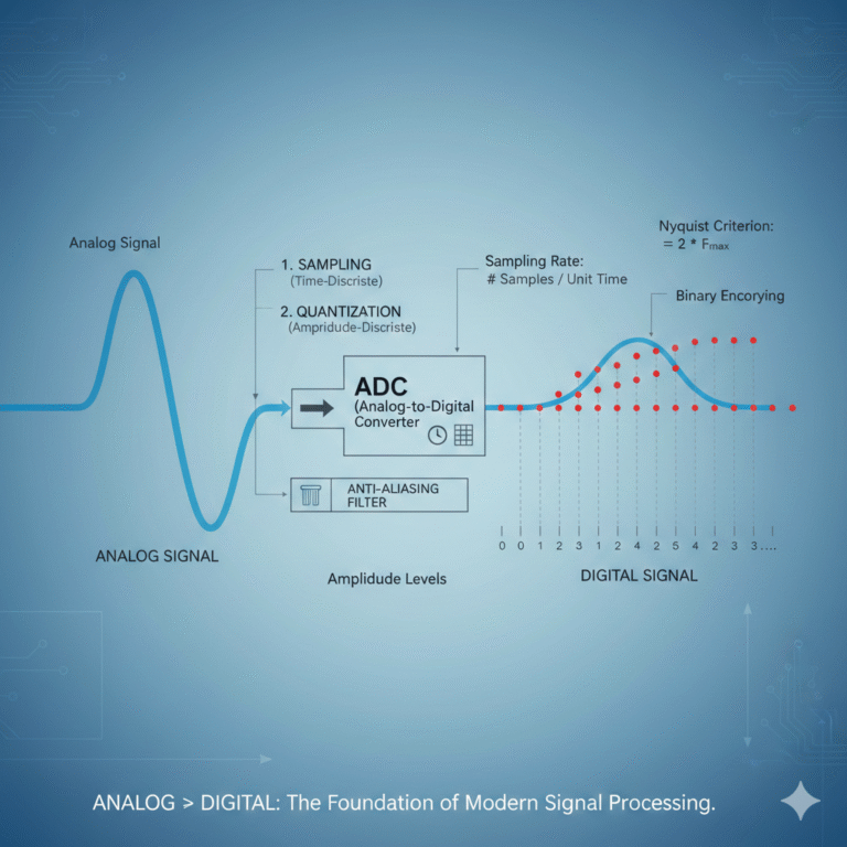
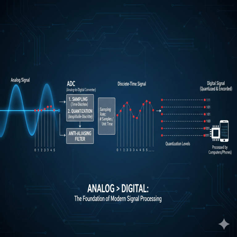
1. What is Sampling?
Sampling refers to the process of measuring and recording a continuous-time analog signal at fixed intervals, thereby converting the continuous-time signal into a discrete-time sequence. Sampling transforms the time axis from a continuous domain into an integer-indexed domain, allowing the signal to be processed by digital systems. The sampling rate is the number of samples taken per unit time, and a higher sampling rate provides higher time resolution and retains more dynamic details.
Before sampling, anti-aliasing filtering must be performed. This is because the frequency spectrum of a discrete-time signal repeats periodically at the sampling frequency. When the input signal contains frequency components exceeding half the sampling frequency, high-frequency components will fold into the low-frequency region and interfere with true low-frequency components, causing irreversible spectral aliasing. Once aliasing occurs, it is impossible to recover the original signal in the digital domain. Therefore, an analog low-pass filter is required before the sampler to limit the input signal within the target bandwidth and eliminate the risk of aliasing at the source.
The sampling rate should meet the Nyquist criterion, which states that the sampling rate must be at least twice the highest frequency component of the signal. Additionally, the sampling rate must align with the system’s data throughput, storage capacity, and real-time computational abilities. Increasing the sampling rate increases the data size linearly and directly impacts backend processing.
2. What is an Analog Signal?
An analog signal generally refers to a continuous signal. It is continuous both in time and amplitude, meaning that between any two adjacent moments, there is a definite value. Thus, it can be completely described by a continuous function.
Real-world phenomena such as sound pressure, light intensity, temperature changes, pressure fluctuations, and variations in voltage and current are all examples of analog signals. These physical processes evolve continuously and do not present discrete jumps.
In measurement systems, an analog signal is not an abstract concept. It is an electrical signal generated after a physical quantity is converted by a sensor and processed by an analog frontend. The effective information range of an analog signal is determined by the sensor bandwidth, frontend frequency response, linear range, and noise floor. Therefore, the analog stage of the system already defines the upper limit of information that can be captured, and subsequent digitization cannot recover bandwidth and details lost in the analog domain.
3. Are Digital Signals and Discrete Signals the Same?
After sampling, a series of data points are obtained, each meaningful only at specific moments. These signals are typically referred to as discrete signals in data acquisition systems. Often, they are also called digital signals, as they already take the form necessary for digital processing.
The transition from an analog signal to a digital signal usually involves an additional step called quantization. While sampling addresses the issue of converting from continuous to discrete in time, quantization addresses the issue of representing amplitude. Quantization maps the sampled values to a finite set of numerical levels, ultimately forming integer encoding that is easier for computers to process.
This entire process is typically carried out by an ADC (Analog-to-Digital Converter). Therefore, it is common to see descriptions that state that an analog signal becomes a digital signal after being sampled, quantized, and encoded by the ADC. Ultimately, the data that a computer or phone processes is a sequence of sample points.
In everyday language, “discrete signals” and “digital signals” are often used interchangeably, especially in data acquisition scenarios, where the sequence obtained after sampling is typically referred to as a discrete or digital signal. People generally do not differentiate between the two terms.
4. Differences Between Analog and Discrete Signals
Imagine a continuous sine wave, for example, a sine signal with a frequency of 10Hz, which repeats 10 times per second. This is a smooth curve on the time axis, representing an analog signal.
If we sample this signal, say by taking 10 points per cycle, then in one second, there will be 10 cycles, and 100 points will be sampled, resulting in a sampling rate of 100 samples per second. The discrete signal will appear as a series of scattered dots on the curve. Many textbooks connect these points with lines for visual convenience, but this line does not represent a true continuous value between the points.
In discrete signals, the “middle value” between points is undefined, so asking “what is the value between the first sample at 0 and the second at 0.59” does not make sense, as there is no defined value between these samples. It’s similar to asking for a number between 1 and 2 in the natural number sequence—there is simply no such value because natural numbers are discrete.

5. Conclusion
The conversion from an analog signal to a digital signal is influenced by four key factors that determine the practical performance limits:
The effective bandwidth of the signal and the anti-aliasing filter’s bandwidth control, as well as amplitude-phase characteristics.
The effect of quantization bit width and full-scale configuration on dynamic range utilization.
The direct limitation imposed by sampling clock jitter on high-frequency precision and signal-to-noise ratio.
The impact of analog frontend noise, linearity, and temperature drift on long-term stability and calibrability.
When all four of these factors meet design specifications, the sequence obtained through sampling forms a reliable digital signal, which can support subsequent digital processing tasks such as filtering, compression, transmission, feature extraction, and intelligent recognition.