PID control is one of the most commonly used strategies in industrial automation for precise process control. A PID controller adjusts system output by computing the error between a desired setpoint and a measured process variable. This adjustment is governed by three core parameters: Proportional (P), Integral (I), and Derivative (D). Understanding the function of each term is essential for tuning the controller to achieve optimal system performance.
1. Proportional Control (P)
The Proportional term determines how strongly the controller reacts to the current error value. Its basic equation is:
ΔP=Kp⋅e
Where:
Kp is the proportional gain,
e is the error (difference between the setpoint and the process value).
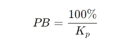
The proportional gain acts as an amplifier. A high gain results in aggressive correction, while a low gain yields a more stable but slower response. However, in most analog controllers, this is expressed as proportional band (PB) rather than gain:
This means:
Smaller PB = Higher gain = More aggressive control.
Larger PB = Lower gain = More stable response.
Limitation: Proportional control alone cannot eliminate the steady-state error, also known as the offset. To address this, the integral term is introduced.
2. Integral Control (I)
The Integral term addresses the steady-state error by accumulating the error over time. When a constant error exists, the integral function increases the controller’s output until the error is eliminated.
ΔPi=Ki⋅∫e(t)dt
Where:
Ki is the integral gain, usually represented as 1 / T_i where Ti is the integral time.
Key concepts:
Smaller Ti = Faster integration = Stronger integral action.
Larger Ti = Slower integration = Weaker integral action.
Effect: Integral control helps eliminate offset but may lead to oscillations or overshoot if not tuned properly. It is almost always used in combination with proportional control.
3. Derivative Control (D)
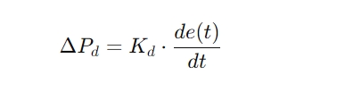
The Derivative term anticipates future error by evaluating the rate of change of the error. It is useful in systems with lag (e.g., thermal systems) and helps reduce overshoot and oscillation.
Where:
Kd is the derivative gain, also represented by the derivative timeTdT_dTd.
Key concepts:
Larger Td = More sensitive to error change.
Smaller Td = Less sensitive.
Effect: It reacts to rapid changes, improving response time. However, if the derivative action is too strong, it can cause spikes or noise amplification—especially if acting on noisy signals. To prevent this, many DCS or modern PID algorithms apply derivative action only to the process variable (PV) rather than the error, reducing output spikes during setpoint changes.
4. Combined PID Output Equation
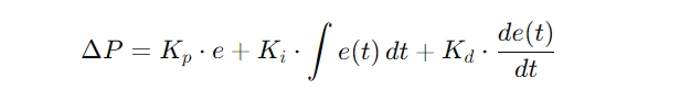
In most controllers, the output is calculated by combining all three actions:
Where the contribution of each term can be adjusted to suit specific process dynamics.
5. Practical Considerations in PID Tuning
Start with P-only control to observe system sensitivity.
Add I to eliminate steady-state error.
Add D to improve response and reduce overshoot, especially for slow-responding processes.
Use tuning methods such as Ziegler–Nichols, trial and error, or model-based tuning for optimal performance.
Always test the controller response under realistic process conditions.
6. Conclusion
PID control remains an essential tool in modern process control systems. By understanding and properly tuning the P, I, and D parameters, engineers can significantly improve system performance, stability, and reliability. Proper use of each component—whether alone or in combination—enables the controller to adaptively handle a wide range of industrial applications, from simple flow loops to complex temperature or pressure regulation.